On being Sensitive and Specific – analytically speaking

In this (technical) post, I illustrate how to calculate commonly used goodness of fit statistics.

Goodness of fit statistics are essential components to doing statistical model building. They are how you tell whether your model is performing well ito explaining the patterns in your data.

In practice, most of these are done automatically from the software you use. However, knowing how these are derived gives you a much deeper level of understanding.

The scenario is that I built a model predicting the number of ED visits among a patient pool. I have an output data set that has

1. the patient ID,
2. whether the patient had ED visits and
3. what the model I built predicted as the probability that the patient had ED visits.

Please download the worksheet as you read this.

 

Step 1: I paste the output data in the spreadsheet

I used a decision tree to build the predictive model. See this post on decision trees

Step 2: I calculate the R-Squared

This is very high level measure of how much data variation is explained away using the predictive model. It’s a useful initial measure to see whether the model you build does any good, in layman terms…

Mathematically, it’s calculating

• A (total no model error): the difference between each data point and the arithmetic average ED rate across all patients, taking the square of that and add across all data points. (column E)
• B (total with model error): the difference between each point and the predicted ED rate for each patient, then take the square of that and add across all data points. (column F)
• R-Squared = 1 – B / A

The higher the R-Squared the better, generally speaking. (Note that R squared ignores non linearity, over fitting, and other important considerations)

Step 3: I calculate the sensitivity vs specificity table

When doing binary outcome prediction, you can get 4 types of outcome when making a prediction.

These measures are then used to calculate a whole lot of statistics which detect how well the model is performing. FP is also called type I error. FN is also called Type II error.

• Sensitivity refers to when the model correctly predicts an ED visit when the patient had ED visits. (TP/(TP+FN))
• Specificity refers to when the model correctly predicts no ED visits when the patient did not have ED visits. (TN/(FP+TN))

I used cell AA8 to specify the cutoff level, so that the average rate of ED visit are close (cells G7 and C7 are close). Concretely, I chose 90% probability above which I decide the prediction was that the patient would have had an ED (1). Below 90% would mean no ED visit prediction (0).

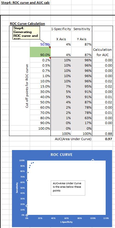
Step 4: I calculate the AUC after generating the ROC curve

ROC (Receiver Operating Characteristic) curve represents how well the model performs in terms of sensitivity and specificity under different cut off points.

I can decide 90% probability is counted as a likely ED visit and below 90% counted as a negative (column G), with a corresponding set of sensitivity and specificity measures (cells AC8 and AB8). I can also use say 60% as the cut off. At different cut off points, different sets of sensitivity and specificity will be generated.

The table (AB10-AC23) represents the set of sensitivity and (1-specificity) measures at 0.2% cut off up to 90% cut off levels. I used a data table to calculate those sensitivity and specificity sets and plotted the 1-specificity and sensitivity points. The area under the points on the ROC curve is referred to as the AUC (Area under curve).

In column AD, I estimated the AUC using linear interpolation (simply, connecting the dots using straight lines and adding up the slices of the area between each dot).

Step 5: I calculated all the Confusion Matrix

Confusion Matrix is a sadistically named set of goodness of fit metrics… The metrics are very useful in gauging how well a model is performing.

I’m not going into detail on these. Suffice to say that these are standard outputs from a Confusion Matrix output using most statistical software packages. Depending on the modeling you’re doing, some of these measures will be more important than others. For example, some predictive modeling requires very high sensitivity, i.e. you predict the disease when the patient has the disease, while other times you will need to have high specificity, i.e. you don’t predict a disease when the person does not have it.

A lot of how to gauge a model’s performance is more art work than science, as there are no perfect models. You would need to know why you’re doing the predictive modeling AND know the models chose to do the predictive modeling well.

Please subscribe to receive future posts similar to this one. Thanks for reading!